HomeAustralian Severe Weather AssociationStormchasing ReportsPhoto GalleriesStorm InformationLinksAssorted Items

Interpreting Skew-Ts (Part Two)

We're going to look at some more examples soon, but first lets learn a little more about this new line - after all, it's probably the most important line of the Skew-T, but you can control it too!  Remember a few things we learnt in the first part of this guide about instability:

- Higher surface temperatures = higher instability (or less stability)
- Higher surface moisture = higher instability (or less stability)
- Colder upper level temperatures = higher instability (or less stability)

Conversely, the opposite is also true for all of these (eg lower surface temperatures produce lower instability and an increase in stability and so forth).

Keeping this in mind, we also know that our TAPP line not only tells us whether the atmosphere is stable or unstable, but also how stable and unstable it is.

So then - do you think that the TAPP line and the surface temperature and moisture, and the upper level temperatures could be related?  If you think yes - you're right!  In fact, if you know the surface temperature and dewpoint, you can plot the TAPP line!  This is extremely important, knowing how to do this gives you full control over Skew-Ts - I know it's a bit of work, but trust me - you'll understand things a lot more if you understand exactly how it works!

Once again, an archived Wyoming sounding is the best illustration of this (I'll get back to the proper BoM soundings the next time - I promise!)


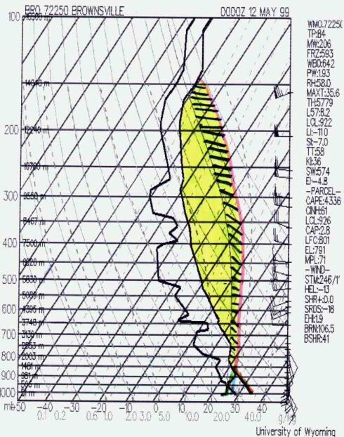
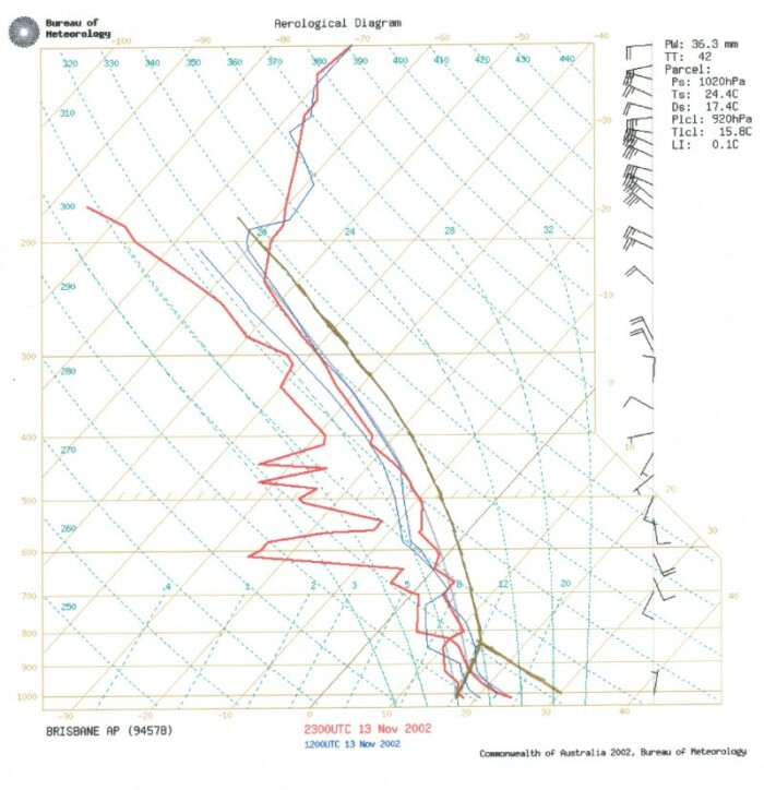
Look how far to the right the air parcel line is to the ELR!!!  The CAPE is calculated at 4336 and LIs -11 – the atmosphere at first glance appears EXTREMELY unstable.  However, technically it isn’t!  Look at the cap near 900mb, that’s a fairly large cap!

Looking at the air parcel line and ELR, air is not going to rise above 950mb, all that CAPE above will simply go to waste.  The atmosphere at this point is “stable.”  However – if certain conditions occur, that cap could ‘break,’ for this reason, the correct terminology is “conditionally unstable.”  Rather – it is conditional upon other variables to whether or not it will be unstable or not.  If cooler air comes aloft near 900mb (and assuming that the warm, humid air at the surface prevails) the cap will decrease significantly, until eventually air at the surface will be allowed free passage through the atmosphere.  Conditionally unstable atmosphere’s generally cause the most severe thunderstorms.  The reason for this, is that all the heat of the day is kept at the surface, and then when the cap suddenly breaks, you have an entire day's heat energy from the Sun to utilise in energy and ‘fuel’ for thunderstorms.  There are a multitude of other ways the cap can be broken, quite frequently it is by added heat at the surface.  If you heat the air up further at the surface, it is more likely to be warmer then the rest of the atmosphere as it rises.  A trigger will also help break the cap, in many situations just heating a conditionally unstable atmosphere isn't quite enough to break the cap, you still need some forcing to help get the initial parcels of air rising.  Here we come into the basics of nowcasting and forecasting CAPE during situations such as these. 

We learnt before that air will cool at the DALR (Dry Adiabatic Lapse Rate) until it reaches 100% humidity (ie saturated), and then from that point it will cool at the SALR (Saturated Adiabatic Lapse Rate).  The point at which this changes is the LCL (Lifted Condensation Level) - ie the base of the clouds.  However, this path changes as heat and moisture at the surface changes.  As heat and/or moisture at the surface increases, the air parcel line is “shifted” to the right.  The LCL also changes as heat and moisture changes.  Both of these points are critical.  But using this information that's been presented, do you think if we added enough heat (or moisture) into the atmospheric situation described by the sounding that we might be able to break the cap?

What do we need to know here to work it out?  Well...we need to know:

a) by how much is the theoretical air parcel plot shifted to the right?  And... 
b) where is the new LCL? 

The relationship can be related by “Normands Theorem.”  This simply states this: 

That the LCL is where the following lines intersect: 

- The DP (Dewpoint) from 1000mb, taken up through the atmosphere following the pattern of a mixing ratio line. 
- The T (Temperature) at 1000mb, taken up through the atmosphere following the pattern of a DALR line. 

Where these two intersect, is where the LCL will lie.  Lets assume that the DP remains the same, but the temperature rises to 35C during the day. 

From the DP, follow a mixing ratio line upwards for a few centimetres.  From the temperature, follow a DALR up for a few centimetres, see where the two intersect?  Tadah!. We have now just found our new LCL!  We can now plot the rest of the Skew-T.  We can now clearly see that the atmosphere has become unstable!  We have also added more CAPE, as we can see the area between the air parcel line, and the ELR has increased considerably.  Our CAPE is now well in excess of 5000!  Not to mention the atmosphere is now unstable, we can now expect some very large (and severe) thunderstorms. 


Above is the new Skew-T with the added heat at the surface.  The green line is from the DP, following a mixing ratio line.  The orange line is the air parcel line from the temperature, following a DALR line, and the red-pink line is a continuation of the air parcel line, after the LCL has been reached, and the air is cooling at the SALR.  The shaded yellow is the CAPE, with the stripped yellow indicating the new CAPE added by increasing the surface temperature.  (NB - Ignore the middle dark black line, this was the old ELR, the new ELR is on the right - as the bottom part of the atmosphere changes temperature somewhat during the day.  Also ignore the blue line drawn in - knowing what this is now obsolete). 

You may be wondering about the changes in temperature in the atmosphere. Anything above 850mb, is not effected by diurnal temperature changes at the surface.  Providing our upper atmosphere remains the same (and fluctuations are common, but generally aren’t significant.  They only occur by temperature advection, and this can be forecasted well in advance by looking at forecast Skew-T’s <which will be mentioned later> and seeing the expected changes in the atmosphere.)  Anything below the 850mb line that changes, is most likely to follow a DALR line.  This means that air will rise slowly at this point, but as soon as it passes the broken cap, it will rise very quickly, and convection will “explode.”

There are limitations of “Normands Theorem” – during very dry situations, and inversions right above the surface, the LCL does not exactly follow this plot.  Because of these limitations, many people tend to alter this process a little.  The next section illustrates how that process is changed to give a more accurate representation of the atmosphere.  Don't worry, it's not difficult at all - in the long run it'll take an extra half a second, but it'll probably save you hours of bust stormchasing!

Finally we have an example of a potentially unstable atmosphere.  That is, it can potentially be unstable if a few things happen.  You might be wondering if this is the same as a conditionally unstable atmosphere.  However a conditionally unstable atmosphere is generally an unstable atmosphere with a moderate to large cap that could potentially be broken.  However, a potentially unstable atmosphere is an atmosphere that is almost completely stable – but only just stable or very marginally unstable (but overall because there's too many stable points, it's generally considered stable.  But a few normal changes that occur during the day could easily cause the atmosphere to become unstable.  Below is a Brisbane sounding for November 14:


Look at the ELR and air parcel line, oh no!  A fair chunk of the air parcel line is to the left or the ELR!  So there's quite a few stable areas with some marginally unstable regions.  Not to fear though!  This Skew-T is taken on Nov 13 at 23z, (Nov 14, 9am local time), but 9am in November (summer in Bris Vegas for those northern hemispheric folk reading this) means there's oodles and oodles of potential heating from sunlight (providing it's not cloudy) yet to come.  We can see here that the plot is taken at approximately 24.4C with a dewpoint of 17.4C.  How did I know it so exact?  Ok, lets look at another thing briefly on the sounding before we go further...

Right, lets make some sense of this (you may have already guessed some of them already going by their abbreviations).
 

PW Precipital water.  If you condensed all the water in the atmosphere above you, then you would get 36.3mm of water (in this example).  The higher this is, the more moisture in the atmosphere.
TT Total total values, click here for more information.
Parcel Below is the parcel information
     Ps Pressure at the surface (1020hPa)
     Ts Temperature plotted at the surface for the TAPP line (24.4C)
     Ds Dewpoint plotted at the surface for the TAPP line (17.4C)
     Plcl Pressure at which the LCL occurs (920hPa), the higher the pressure the lower the bases of convective development.
     Tlcl Temperature at which the LCL occurs (15.8C)
     LI Lifted index value, click here for more information.

Now that that is out of the way, lets look at replotting our sounding!  We know it's going to be warmer than 24.4C!  Moisture?  Hmm...lets keep it constant for now for simplicity, but remember that moisture can also change!  Lets say it gets to 30 degrees and moisture stays the same.  If we follow our rules of Normands Theorem as before, we can arrive with a new air parcel plot, that has all of the air parcel line to the right of the ELR! 

You can now see that the atmosphere is clearly unstable.  Not hugely unstable (LIs are -2 at 500mb, remember the rule to calculating them?  If not, click here.  But if we work out the maths:

-10C - -8C = -2LIs

Also note that it is fairly consistently unstable throughout the atmosphere - that's good, there's some good moderate instability here!  Not too bad given the sounding initially didn't suggest any convection!  That's a critical thing to remember, and I'll discuss that more in the following section.  Were there severe storms?  A little further south there were some one foot hail drifts - in SE QLD not so much, look at the shear, barely 20 knots until above 300mb!  The shear section of this guide helps describe why it's difficult to get severe storms in that type of shear and proposes some better shear values that we might want to look for.  Check out the chase report of this day though if you're not convinced there were storms!

Now that we have learnt how to re-plot skew-t’s with different surface conditions, and read instability/stability – we can now continue to really let Skew-Ts do some work for us!